For those interested, this article will cover how I use my dataset to built a machine learning model and accurately predict games, as well as some insights into the models. Note that the the most tedious part of the process will not be covered in this article, which consists of scraping the right stats for the model and arranging it into a good dataset, cleaning the data, and making it ready to be input into a machine learning model.

Step 1: Making the data ready to be inputted into a machine learning model

#read the dataset into a pandas dataframe
dataset = pd.read_csv('full_dataset_week4-16_2007-20.csv',index_col=False)
inputs = dataset.drop(columns=['away_team','home_team','home_win','result_diff', 'spread','Unnamed: 0','home_score','away_score'])
print('input size' + str(inputs.shape))
#after removing the columns from the dataset I do not care about, the rest will be used as inputs into the model
inputs = inputs.to_numpy()
#the "target" (what the model is trying to predict) is whether the home team wins or not 
outputs= dataset.home_win
        
print(outputs.shape)
#splitting data into test set 
#Two options: split randomly OR use two/three seasons as test set
use_single_season_as_test = True
number_seasons = 2
games_to_use = number_seasons*194
if use_single_season_as_test:
    endpt = inputs.shape[0]-games_to_use
    X_train = inputs[0:endpt,:]
    X_test = inputs[endpt:inputs.shape[0],:]
    print(X_train.shape)
    print(X_test.shape)
    y_train = outputs[0:endpt]
    y_test = outputs[endpt:inputs.shape[0]]
    print(y_test.size)
else:
    X_train,X_test,y_train,y_test = train_test_split(inputs,outputs,test_size=0.15,random_state =22)
#try both min max and standardization
norm0 = MinMaxScaler().fit(X_train) 
norm1 = MinMaxScaler().fit(X_test) 
X_train_norm = norm0.transform(X_train)
X_test_norm = norm1.transform(X_test)
#this makes sure the labels are binary (either 1 or 0)
lab = LabelEncoder()
y_train = lab.fit_transform(y_train.ravel())
y_test = lab.fit_transform(y_test.ravel())

The block of code above reads the data into a dataframe and sorts it into the inputs and outputs to be fed into the model.

Then, I split the data into training and test data. Test data is pivotal in machine learning to backtest your model, as if you only use the same data the model is trained with to figure out the accuracy of the model, there will be a large inherent bias in those results.

I have two options for the test data: either taking a random split, or picking 2 full seasons of NFL data from week 4-16. I have experimented with both methods shown below: randomly shuffling the entire dataset then splitting it into test data, or using the last 2 seasons from the dataset. The latter allows insights into whether over over the course of a full season the model built is profitable or not, so I will choose this for now. Note that the model is profitable either way, this is just for demonstration purposes.

My outputs and target is whether the home team won or not in this example. a 1 would indicate a home win, and a 0 would indicate a home loss. Note that in my real models I have slightly more complicated outputs but this was simplified for demonstration purposes.

Finally, I use a technique called min-max scaling. The purpose of this is to optimize how well the model is able to learn (and how quickly as well). If you have, for example, a set of 20 inputs and some range from 0-100 while some range from -1 to 1, the models will find it harder to learn, to put simply. For more information on this, check this article out. Now the data is ready to be inputted into machine learning algorithms!

Step 2: Feature Selection

X_train_norm_mod = pd.DataFrame(X_train_norm, columns = [THESE ARE THE NAMES OF EACH STAT I HAVE IN MY DATASET (OVER 100+])
#use sklearn in built model that recursively goes over every combination of features and selects only the ones that have predicitive correlation with the target data
rfecv = RFECV(estimator=LogisticRegression(solver='liblinear'),min_features_to_select=6,step=5,n_jobs=-1,scoring="precision",cv=5)
rfecv.fit(X_train_norm_mod, y_train)
X_train_norm_mod.columns[rfecv.support_]

I will not be sharing the inputs as this is what causes the model to be so accurate. After hundreds if not thousands of hours of work on this, I have deduced that only by using a very specific set and combination of stats from the NFL is a model able to best the sportsbook ones, and even then it is only truly profitable after 3 full weeks of play. I will say though, that the inputs are not based on any future data, meaning if the inputs are from a 2011 game played in week 6, the inputs are based on only information available at week 6 and before.

The code does show that in-built libraries (like SKlearn, which is being used here) make it really easy to build a model that incorporates feature selection.

This method of feature selection essentially recursively loops through every combination of all the inputs given, and selects only the ones that have predictive capability to the target. Simply put, it picks only the stats which help predict whether the home team will win or not.

I am using a base logistic regression model in built with SKlearn, and the interesting thing is that instead of optimizing for accuracy, I am optimizing for precision. The reason for this is that when trying to bet based upon future results, I obviously do not know the result ahead of time. But if the model has high precision, I can be confident that whatever result is predicts is accurate. Now there is no “right” answer, optimizing for accuracy is not a bad thing either; with the dataset I have, I have found that this is what leads to the highest profits.

The last line will simply name the features that the model has selected.

Step 3: Using a more refined logistic regression

#training model with ALL features using a more complex log reg model
#Note: this actually uses Keras, but SKlearn can be substituted
X_train_selected = X_train_mod[X_train_norm_mod.columns[rfecv.support_]]
model = Sequential()
nu_inputs_model = np.size(X_train_selected,1)
model.add(tf.keras.Input(shape=(nu_inputs_model,)))
#this adds regularization techniques, which help improve the machine learning model
model.add(Dense(units = 1, activation='sigmoid',kernel_regularizer=regularizers.l2(l2=1e-4)))
model.compile(Adam(lr=0.0001), 'binary_crossentropy', metrics=['accuracy'])
h = model.fit(x=X_train_selected, y=y_train, verbose=1, batch_size = 64, epochs = 2000, shuffle = 'true', validation_split=0.15)

All that’s being done here is I take only the subset of features selected in the previous step, and create a slightly more complicated logistic regression model in which I have manually tuned some of the hyper-parameters (this is a fancy name in machine learning for the parameters you decide, like the number of epochs). I have chosen a very low learning rate with a high number of epochs as this is what I have found leads to the best results with this model. Note that the models used to generate the actual picks is much, much more complicated than this (I use a non-conventional neural network architecture called Generalized Additive Network as a base model, although it is slightly modified) but the basic overall steps are the same.

The validation data is a subset of the training data held back from the training data every epoch that is used to backtest the data every epoch. Every epoch, a random 15% (as I defined 15% in the code above) gets taken out and tested out, to ensure the model is not just overtraining. Overtraining is essentially when the model weights are so optimized for the training data that it would be unable to properly predict any data outside what it was trained on, which is the whole purpose of a neural network.

Step 4: Looking at the results from the model

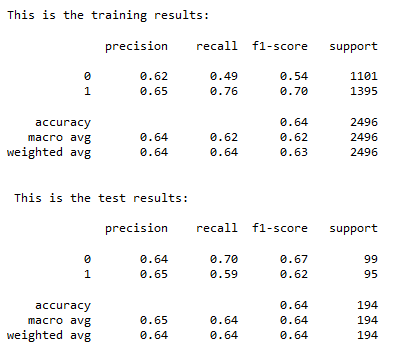
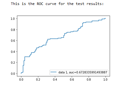
All the model success really boils down to is its ability to profit over the course of a full season or two, which will be shown shortly.

Note that I mentioned in a previous article that to make profit, the generalized number should be around 66%. This model is actually slightly lower than that number but still leads to high profit margins. This is because it is able to predict a large number of upsets overall, so the average return from each bet staked is high enough to combat the (relatively) lower accuracy. This is the interesting trade off when it comes to building models for sports betting, as a higher accuracy model does not directly correlate to more profit!

Step 5: Simulating a set of bets with the test data and outputting the profit

As mentioned in a previous article, for classification models, the way to turn probabilities into how much to bet is based on the kelly criterion, so the code for this is below:

#prob model is a prediction from a trained model
#odds is the corresponding odds you from the sportsbook for the game
#initialbankroll is what u start out with
#winorloss is whether you would have won the bet
#scale down factor is just conservative value 0<value<1 to decrease bet sizes if being conservative
def compute_and_eval_kelly(prob_model,odds,initial_bankroll,win_or_loss,scale_down_fac,debug_kelly):
    if odds>0:
        sportsbook_return = abs(odds)/100
    else:
        sportsbook_return = 100/(abs(odds))
    K = ((prob_model*sportsbook_return) -(1-prob_model))/sportsbook_return #kelly formula
    #print(K)
    if K>0: #only bet if kelly is positive
        bet_size = scale_down_fac*K*initial_bankroll #scale down kelly to be more conservative
        
        #this means model correctly predicted result
        if win_or_loss: 
            new_bankroll = initial_bankroll + (bet_size*sportsbook_return)
            if debug_kelly:
                print('Win!')
                print('New Bankroll is' + str(new_bankroll))
            return new_bankroll           
        #this means model incorrectly predicted result
        else:
            new_bankroll = initial_bankroll - bet_size
            if debug_kelly:
                print('Lost')
                print('New Bankroll is' + str(new_bankroll))           
            return new_bankroll
    else:
        if debug_kelly:
            print('No bet placed..')
        return initial_bankroll #not placing a bet on this game

This “simulates” a bet based on the probability from the model, the corresponding ML odds, and computes a new bankroll based on whether the bet would have won or lost. Note that I have added a conservative factor, because as I mentioned the kelly criterion sometimes leads to aggressive bets in a previous article; it is best to find a lower number which still leads to profit while lowering the risk. That is what the variable “scale_down_fac” does.

There is also some print statements in this function just to ensure the math was being done correctly, but this is not necessary.

Then, I have built another function to simply loop through all the test set and compute the final bankroll from the initial one, simulating every single bet in the test set. In the case shown, remember the test set consists of 2 full seasons of NFL games ranging from week 4-16. I also loop through the “conservative” factor to find the most optimal balance between risk and profit.

# -*- coding: utf-8 -*-
"""
Created on Sun Sep 11 17:02:55 2022
@author: sashe
"""
from Kelly_Critereon import compute_and_eval_kelly
import numpy as np 
def KellyReturn(X_FK,ML_FK,Y_FK,Truth_FK,kelly_loop,debug_kelly):
    if kelly_loop:
        kelly = np.linspace(0,1,100)
        ROI_vec = np.zeros([100,1])
        for k in range(0,np.shape(kelly)[0]):
            kelly_scaledown = kelly[k]
            bankroll = 1
            model_correct_tmp = []
            #np.shape(X_test_norm)[0]
            #print('loop' + str(k) + '\n\n')
            for i in range(0,np.shape(X_FK)[0]):
                if (Y_FK[i]>0.5 and Truth_FK[i]==1) or (Y_FK[i]<0.5 and Truth_FK[i] ==0):
                    model_correct_tmp.append(1)
                else:
                    model_correct_tmp.append(0)
                if (debug_kelly):
                    print('model probability was: ' + str(Y_FK[i]))
                    print('ML odds were: ' + str(ML_FK[i]))
                    print('Model was right: ' + str(model_correct_tmp[i]))
                bankroll = compute_and_eval_kelly(Y_FK[i],ML_FK[i],bankroll,model_correct_tmp[i],kelly_scaledown,debug_kelly)
            ROI = (bankroll-1)*100
            ROI_vec[k] = ROI
            #print('Return on investment is: ' + str(ROI) + '%')
        return ROI_vec
    else:
        kelly_scaledown = 0.3
        bankroll = 1
        model_correct_tmp = []
        #np.shape(X_test_norm)[0]
        for i in range(0,np.shape(X_FK)[0]):
            if (Y_FK[i]>0.5 and Truth_FK[i]==1) or (Y_FK[i]<0.5 and Truth_FK[i] ==0):
                model_correct_tmp.append(1)
            else:
                model_correct_tmp.append(0)
            if (debug_kelly):
                print('model probability was: ' + str(Y_FK))
                print('ML odds were: ' + str(ML_FK[i]))
                print('Model was right: ' + str(model_correct_tmp[i]))
            bankroll = compute_and_eval_kelly(Y_FK,ML_FK[i],bankroll,model_correct_tmp[i],kelly_scaledown, debug_kelly)
        ROI = (bankroll-1)*100
        print('Return on investment is: ' + str(ROI) + '%')
        return ROI
    

The final profit curves from the trained model:

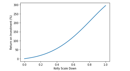
The curve also shows another important trait, as earlier I mentioned the option of scaling down the bets to lower the overall risk. The shape of the line is exponential but becomes linear towards the end, so if one was to be more conservative with their bets, a good “scale down” factor for each bet would be right where the line stops being exponential and starts being linear, which can be eyeballed to be around 0.7.

Note that my models generated with more complex architectures are able to reach around double this profitability mark from a much simpler neural network, the purpose of this article was just to show how I go from start to finish!